Project 1 · Decision Tree: Stock Momentum
This is where the course meets the market. The brief: predict whether a stock's next three months will be Bullish, Neutral or Bearish — and hand the trading desk rules it can actually read. Eight real stocks (Apple to Walmart, 2020–2026, 13,560 trading days), seven technical indicators engineered from raw prices, a tuned decision tree, and an honest scoreboard. Along the way this lesson teaches the finance behind every indicator (what RSI really measures, why a golden cross matters, what ATR says that direction doesn't), reads the code line by line, and hunts three genuine landmines hiding in the original project template — including one that mislabels stocks with their neighbours' future prices. The punchline is an honest number: 46% test accuracy against a 34% baseline, and the reasons why that gap — not a bigger one — is exactly what efficient markets predict.
🎯 Learning Objectives
- Read the five core technical indicators as a trader does: RSI, MACD, moving-average crossover, ATR and volume — formula, intuition, and what each one catches
- Engineer those indicators in pandas, line by line —
diff,rolling,ewm,shift— without leaking the future or bleeding across tickers - Build honest momentum labels from forward 3-month returns, and understand why quantile thresholds redefine "Bullish" as top-third, not "went up"
- Tune a decision tree with Chapter 31's grid-search discipline and read the winner (and its plateau)
- Translate precision, recall and the confusion matrix into trading language — hit rates, missed rallies, false alarms
- State the honest limits: why 46% beats 34% but embarrasses the template guide's 65–75% hope, and the three fixes (walk-forward splits, scaled indicators, real fundamentals) that would earn the next points
1. The Brief
The desk's question, in trader language: "Every morning I see
RSI, MACD, the moving averages, volume. Which combinations of those
numbers actually precede a good next quarter — and can you show me
the rule?" That last clause is why this project is a
decision tree and not a neural network: Chapter 16's
tree is the model whose entire logic can be printed on one page
(export_text) and argued over in a meeting. A desk
can't interrogate 127 weights; it can interrogate
"if ATR ≤ 6.94 and the 50-day average is above the 200-day, then…"
The plan, and where each course chapter plugs in:
| Stage | What we do | Course backbone |
|---|---|---|
| 1 · Data | Daily OHLCV for 8 large-cap US stocks, 2020-01-02 → 2026-09-30 (13,560 rows) | Ch 3's audit discipline |
| 2 · Features | 7 technical indicators engineered per ticker | this lesson §2–3 |
| 3 · Labels | 3-month forward return split into terciles → Bearish / Neutral / Bullish | Ch 3 (leakage) |
| 4 · Model | Decision tree, 120-configuration grid search, 5-fold CV | Ch 16 + Ch 31 |
| 5 · Evaluation | Accuracy vs baseline, per-class precision/recall in trading language | Ch 18 |
| 6 · Interpretation | The rules, the importances, and what the tree got right and wrong | Ch 16 · Ch 17 preview |
The eight stocks — AAPL, MSFT, GOOGL, TSLA, JPM, XOM, JNJ, WMT — are deliberately cross-sector (tech, banks, energy, healthcare, retail) so the model cannot quietly become a sector bet. One honest design note carried over from the original project: the template's "fundamental" columns (P/E, ROE, growth, leverage…) are random placeholders, not real data — and §7 turns that flaw into one of the lesson's best experiments.
2. The Finance Primer — Reading a Chart Like an Analyst
Nothing in this section is machine learning. It is the vocabulary the rest of the lesson speaks — the five indicator families a technical analyst watches every morning, each reduced to one formula, one intuition, and one thing it catches that the others don't.
2.1 RSI — the momentum thermometer (0–100)
By hand, because the course always computes one first. Fourteen daily price changes:
| Sum | Average (÷14) | |
|---|---|---|
| Gains (+1, +1, +2, +1, +2, +2, +1, +2, +1, +2) | 15 | 1.071 |
| Losses (−1, −1, −1, −1) | 4 | 0.286 |
2.2 MACD — trend, with a memory
2.3 The moving-average crossover — the golden cross
When the 50-day average crosses above the 200-day average
("golden cross"), medium-term buyers have overtaken long-term ones —
a classic bull signal; the reverse is the "death cross". The feature
is binary: MA_Crossover = 1 when
SMA₅₀ > SMA₂₀₀, else 0. It is the
slowest, most forgiving signal on the page — and the one with the
longest warm-up (199 days of history before SMA₂₀₀
even exists).
2.4 ATR — how violent, not which way
2.5 Volume ratio — conviction
Price moves on unusually heavy volume carry more information than the
same move on thin volume: someone big is acting.
Volume_Ratio = today's volume ÷ 20-day average volume
— 1.0 is an ordinary day, 2.0 means twice the usual crowd showed up.
The last technical feature, Volatility (20-day rolling
standard deviation of close), is ATR's cousin measured on closes
alone.
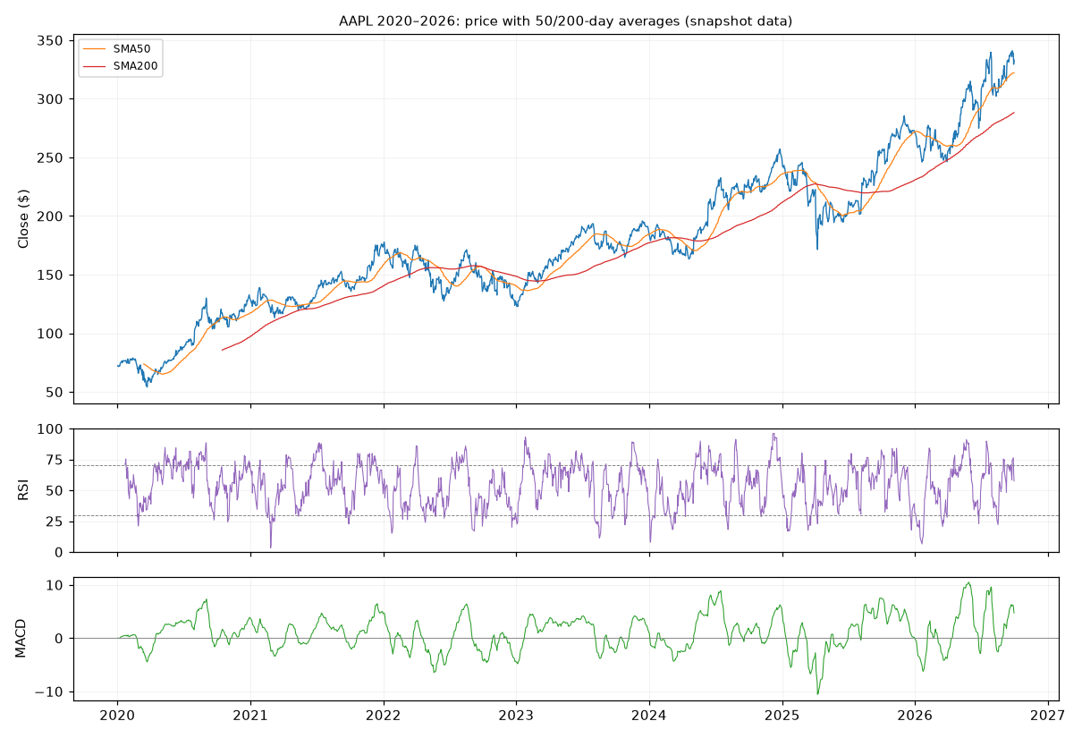
2.6 The fundamental side — what the placeholders would have meant
The project template carries eight fundamental columns as random noise. Real versions would read like this to an analyst — and §8 discusses why using them properly is harder than it sounds:
| Metric | Definition | The analyst's question |
|---|---|---|
| P/E ratio | price ÷ earnings per share | how many years of current earnings you're paying for — is the stock expensive? |
| ROE | net income ÷ equity | how much profit does each unit of shareholders' capital generate? |
| Earnings growth | YoY % change in earnings | is the business accelerating? |
| Debt-to-equity | total debt ÷ equity | how leveraged — who gets paid first in a downturn? |
| Dividend yield | annual dividend ÷ price | cash return now vs growth later |
| Profit margin | net income ÷ revenue | pricing power and cost discipline |
| Current ratio | current assets ÷ current liabilities | short-term solvency |
| Revenue growth | YoY % change in sales | top-line momentum before earnings "management" |
3. From Prices to Features
The engineering loop runs per ticker — that word "per" is load-bearing (§4 explains what breaks without it). The complete, corrected feature block:
for ticker, g in df.groupby('Ticker'):
    g = g.sort_index().copy()                     # one ticker's history, in date order

    # trend
    g['SMA50']  = g['Close'].rolling(50).mean()   # 50-day simple moving average
    g['SMA200'] = g['Close'].rolling(200).mean()
    g['MA_Crossover'] = (g['SMA50'] > g['SMA200']).astype(float) \
                          .where(g['SMA200'].notna())   # NaN while SMAs warm up

    # momentum
    delta = g['Close'].diff()                     # day-over-day change
    gain  =  delta.where(delta > 0, 0).rolling(14).mean()
    loss  = (-delta.where(delta < 0, 0)).rolling(14).mean()
    g['RSI'] = 100 - 100 / (1 + gain / loss)
    g['MACD'] = g['Close'].ewm(span=12).mean() - g['Close'].ewm(span=26).mean()
    g['Momentum'] = g['Close'].pct_change(20) * 100      # 20-day % price change

    # volatility
    tr = pd.concat([g['High'] - g['Low'],
                    (g['High'] - g['Close'].shift()).abs(),
                    (g['Low']  - g['Close'].shift()).abs()], axis=1).max(axis=1)
    g['ATR'] = tr.rolling(14).mean()
    g['Volatility'] = g['Close'].rolling(20).std()

    # volume
    g['Volume_Ratio'] = g['Volume'] / g['Volume'].rolling(20).mean()
Listing 1 — Technical feature engineering, per ticker. Seven features from five columns.
Four pandas idioms do all the work, and each is worth reading slowly:
.diff()— subtracts the previous row: daily price change. The seed of RSI..rolling(n).mean() / .std()— a sliding n-day window; the first n−1 rows have no answer and become NaN. SMA₂₀₀ needs 199 prior days — the per-ticker warm-up that trims our dataset from 13,560 rows to 11,464..ewm(span=n).mean()— the exponential moving average: every row gets a value from day one (weights just decay into the past), which is why MACD has no warm-up but SMA₂₀₀ does..shift()— moves a series by one row; used here to fetch yesterday's close for the true range. Its negative sibling.shift(-63)fetches the future — the entire labelling mechanism, and the entire leakage risk, of §4.
One real row of the finished matrix, so the features stop being abstractions — AAPL, 25 January 2022:
| RSI | MACD | MA_Crossover | Momentum | ATR | Volatility | Volume_Ratio | → Label |
|---|---|---|---|---|---|---|---|
| 15.3 | −2.21 | 1 | −11.4% | 4.37 | 6.37 | 1.25 | Bearish (fwd −1.7%) |
Read it like the analyst who lived it: deeply oversold (RSI 15), below trend on MACD, still technically in a golden-cross regime — and the 20-day momentum had gone decisively negative. The next quarter lost a further 1.7%. One row, seven numbers, one label: that is the entire supervised-learning contract of this project, times eleven thousand.
4. Labelling the Future — Carefully
Supervised learning needs ground truth, and for momentum the truth arrives three months later. The label for day t is built from the price at day t+63 (three months of trading days):
Then the continuous forward return becomes a class. The template uses terciles — the 33rd and 67th percentiles of the whole dataset's forward returns:
| Class | Rows | Mean forward return | Median |
|---|---|---|---|
| Bearish (bottom third) | 3,931 | −9.2% | −7.3% |
| Neutral (middle third) | 3,864 | +5.3% | +5.1% |
| Bullish (top third) | 3,669 | +22.5% | +18.5% |
A 31.7-point spread between class means — that is the prize the tree is trying to rank. And tercile labelling keeps the classes nearly balanced by construction (34.3% / 33.7% / 32.0%), so accuracy's majority baseline sits at 0.343 — the number every result in §6 must beat.
4.1 Three landmines in the template
The original project code ships with three genuine bugs around this labelling step. None of them crash — which is precisely why they are worth studying. All three were found by auditing, and all three are fixed in this lesson's canonical run.
-
The cross-ticker seam. The template concatenates
all tickers into one frame and then calls
shift(-63)androlling(50). Rolling windows and forward shifts run straight across ticker boundaries: Apple's last trading days would be labelled with Microsoft's future prices, and its "50-day average" at the seam mixes two stocks' prices. Fix: every window and shift insidegroupby('Ticker'). -
NaN swallowed into "Neutral". The last 63 days of
each ticker have no future price, so their forward return is NaN.
The template's
np.where(fwd <= lo, 'Bearish',
                    np.where(fwd >= hi, 'Bullish', 'Neutral'))
sends NaN to the else-branch — NaN comparisons are False — quietly manufacturing ~500 fake "Neutral" labels for days whose truth is unknown. Fix:pd.cut, which maps NaN to NaN, then drop the unknowns (504 rows). -
The fake golden cross. During the 199-day SMA200
warm-up,
(SMA50 > SMA200)compares NaN to NaN — which is False — soMA_Crossoverreads 0 ("death cross") for the first year of every ticker, when the honest value is "don't know". Fix:.where(g['SMA200'].notna())keeps those rows NaN until the average exists.
Together the three fixes shrink the dataset from the template's effective 13,400 rows to 11,464 honest ones — the difference between 1,936 rows of contaminated or fake-label data and a clean slate. Chapter 31's lesson generalises: the bugs that cost you are the ones that don't raise exceptions.
5. The Model — Tuned Like Chapter 31 Taught
The classifier itself needs no re-teaching — Chapter 16 built trees from Gini impurity up, and Chapter 31 supplied the tuning discipline. What matters here is the grid, run for real on the 8,598-row training set:
param_grid = {
    'max_depth':        [3, 4, 5, 6, 7],      # five depths
    'min_samples_split':[10, 15, 20, 30],     # × four split floors
    'min_samples_leaf': [5, 10, 15],          # × three leaf floors
    'criterion':        ['gini', 'entropy'],  # × two impurities
}                                   # = 120 configurations

grid = GridSearchCV(DecisionTreeClassifier(random_state=42),
                    param_grid, cv=5, scoring='accuracy', n_jobs=-1)
grid.fit(X_train, y_train)         # 120 × 5 = 600 fits, all cores
Listing 2 — The tuning grid: 120 candidates × 5-fold CV.
| Rank | CV accuracy | criterion | max_depth | min_samples_leaf | min_samples_split |
|---|---|---|---|---|---|
| 1 | 0.4660 | gini | 7 | 10 | 10 |
| 2–4 | 0.4660 | same depth/leaf, split floor 15 / 20 / 30 — indistinguishable | |||
| 5 | 0.4646 | gini | 7 | 5 | 20 |
Chapter 31's plateau, transplanted to finance: the top five candidates sit within 0.0014 of each other, the winner chose the shallowest impurity (gini) and the deepest depth offered (7) — and the split/leaf floors barely matter once leaves hold ≥10 trading days. A depth-7 tree with minimum-10-sample leaves is the champion: 82 leaves, each averaging about 105 training rows. When the top of the grid is flat, any resident of the plateau ships.
6. The Scoreboard
The tuned tree meets the 2,866 held-out days exactly once (Chapter 31's rule). The headline first, then the anatomy:
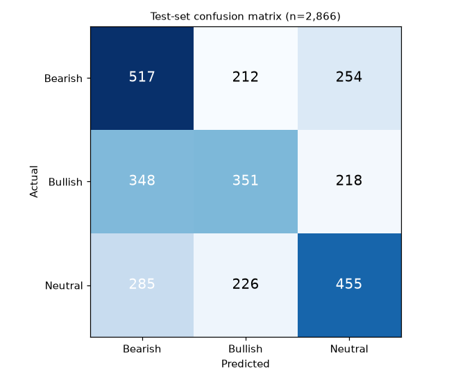
Now the metrics in the only language that matters on a desk — what does betting on this signal cost me?
| Class | Precision | Recall | The trading translation |
|---|---|---|---|
| Bullish | 0.445 | 0.383 | Of days flagged Bullish, 44.5% actually landed in the top third — the "hit rate" of a long signal. Of the true top-third days, we caught 38.3%. |
| Bearish | 0.450 | 0.526 | Half of the genuinely worst days were flagged (decent warning system); but 55% of "sell" flags were false alarms — costly if you exit on them. |
| Neutral | 0.491 | 0.471 | The middle third is where signal goes to die — expected, since it is the class with the least defining character. |
And the single most expensive cell in Figure 3, read as a trade: 348 genuinely Bullish days were labelled Bearish. If the desk had shorted (or simply sat out) on those signals, it missed or bet against days that averaged +22.5% over the following quarter. Precision on the Bearish call and recall on the Bullish call are where the money lives — exactly the class-asymmetric costs Chapter 18 taught us to price before deploying anything.
7. A Trader Reads the Tree
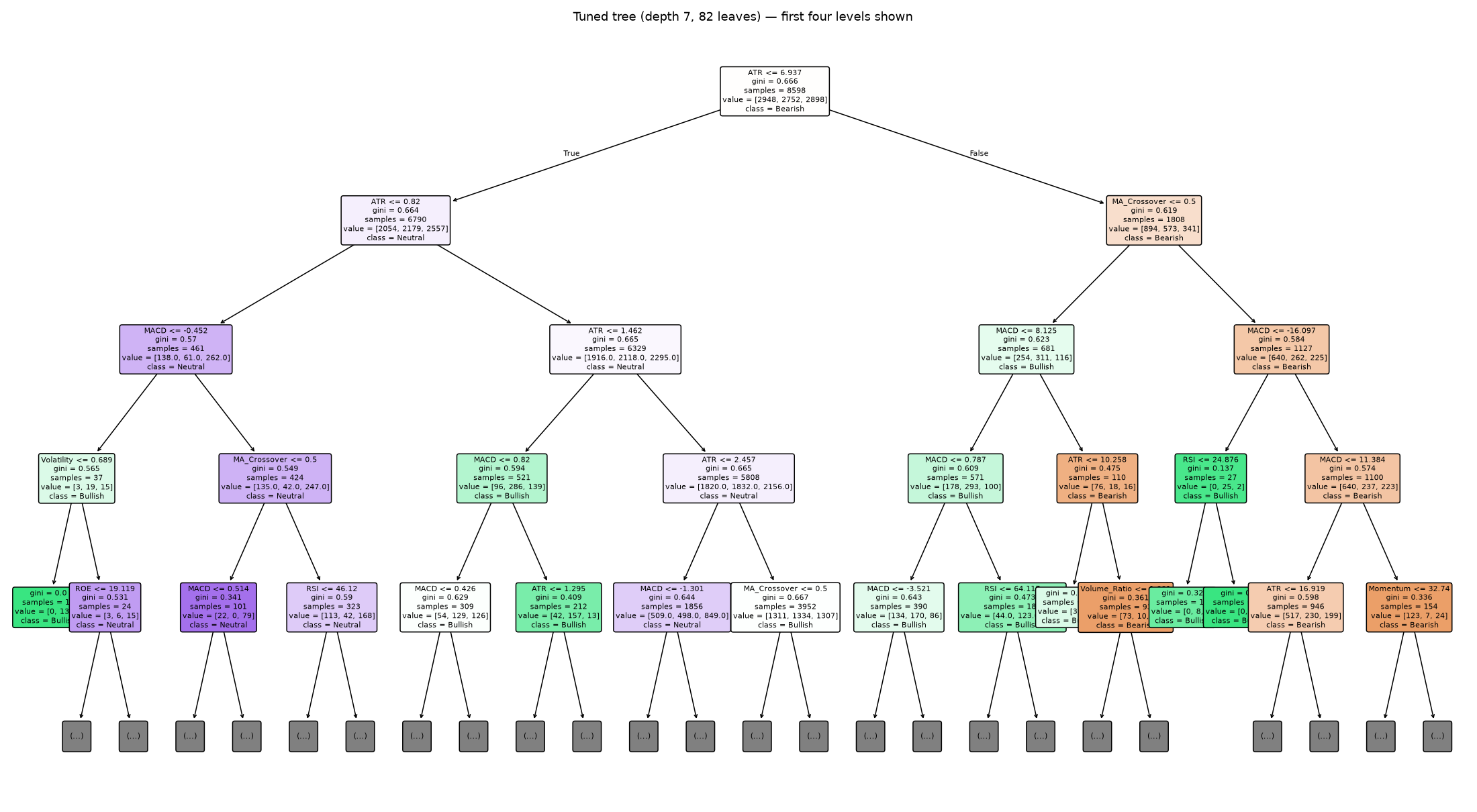
The whole point of choosing this model: its logic can be printed. The champion's first three levels (the full tree is depth 7 with 82 leaves — Figure 4):
|--- ATR <= 6.94
|   |--- ATR <= 0.82
|   |   |--- MACD <= -0.45
|   |   |   |--- Volatility <= 0.69:  class: Bullish
|   |   |   |--- Volatility >  0.69:  [deeper]
|   |   |--- MACD > -0.45
|   |   |   |--- MA_Crossover <= 0.50: [deeper]
|   |   |   |--- MA_Crossover >  0.50: [deeper]
|   |--- ATR > 0.82 ... (calm-regime branches)
|--- ATR > 6.94
|   |--- MA_Crossover <= 0.50
|   |   |--- MACD <= 8.12 ...
|   |--- MA_Crossover > 0.50
|   |   |--- MACD <= -16.10:  class: Bullish
|   |   |--- MACD > -16.10 ...
Listing 3 — export_text(best_tree, max_depth=3), abbreviated. The tree's first question is about violence, not direction.
A trader's reading: the tree's first question is "how violent is this stock?" — ATR at the root — and only then does it ask about trend (MACD, golden cross). Even the counterintuitive leaf helps teach: in the high-ATR branch, days with extremely negative MACD (≤ −16, a severe drawdown) resolve to Bullish — the tree rediscovering mean-reversion inside turbulence: after a violent fall, the next quarter is more often a top-third outcome than a bottom-third one. Rules you can argue with are the product; that is why this project is a tree.
7.1 What mattered — and the noise experiment
| Feature | Importance | Reading |
|---|---|---|
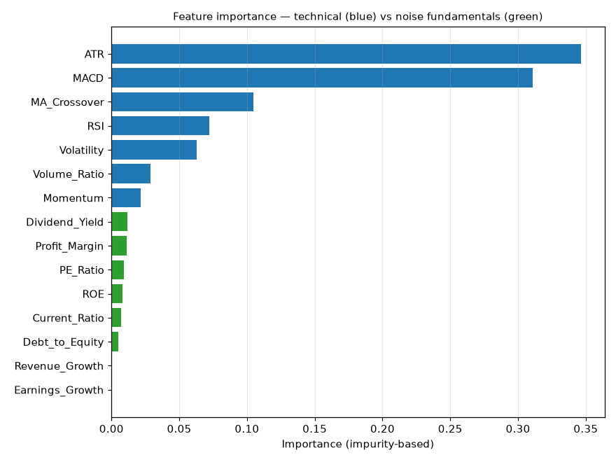
| ATR | 0.346 | v volatility regime is the single strongest clue to the next quarter |
| MACD | 0.311 | trend, with the two together carrying two-thirds of the tree's decisions |
| MA_Crossover | 0.105 | the golden cross earns its keep, modestly |
| RSI · Volatility · Volume_Ratio · Momentum | 0.072 · 0.063 · 0.029 · 0.022 | supporting cast |
| all eight noise "fundamentals" | ≤ 0.012 each | Earnings_Growth: exactly 0.0000 |
The green bars are the lesson inside the lesson. The template's fundamental columns are random numbers, drawn uniform — and the tree, given fifteen features, allocated essentially zero decision weight to all eight of them (largest share 1.2%, one feature literally never used). Information gain cannot be counterfeited: if a column carries no mutual information with the label, splitting on it buys nothing. Replace those green bars with real, point-in-time fundamentals and the chart becomes the genuine experiment — does value+quality data add to what the chart already knows? That is the open door this project leaves for its Random Forest sequel.
8. Honest Limits — and the Professional Upgrades
The original assignment guide told students to expect 65–75% accuracy. Our tuned, bug-fixed, real-data tree scored 46.2% against a 34.3% baseline. Both numbers are correct — and the gap between expectation and reality is the most valuable content in this lesson. Why so hard?
- The market is mostly efficient at this horizon. Three-month ahead ranks are close to the information frontier of public chart data. A 12-point lift over baseline is not a failure; it is the honest size of the edge that seven technical indicators contain. (Enough to be interesting; nowhere near enough to trade unlevered and unhedged after costs.)
- Random splits flatter the model. Training on 2024–2026 rows while testing on 2020 rows lets the tree "know" regimes it shouldn't. Time-ordered evaluation would very likely shave points off — which is exactly why it must be done before believing any backtest.
- Dollar-scaled features leak ticker identity (the warning in §7). Part of ATR's 0.35 importance is stock-selection, not regime-reading.
- No transaction costs, no slippage, no shorting constraints — the label is a return tercile, not a tradable P&L. The capstone's money-metric discipline has not been applied here yet.
The upgrade list, in order of expected payoff:
- Walk-forward split: train ≤ 2023, validate 2024, test 2025–26; then roll. Turns the evaluation from "can it memorise regimes" into "could it have made money in sequence".
- Scale-free features: ATR/Close, MACD/Close, Volatility/Close. One-line change, removes the ticker-identity leak.
- Real point-in-time fundamentals: P/E and ROE as they were on the day — not today's ratios pasted onto history, which would be textbook look-ahead bias (Chapter 3's rule wearing a valuation costume).
- More names: 30–50 stocks (the guide's own advice) — more cross-sectional variety, less single-name regime risk.
- An ensemble: the Random Forest on identical features is this project's designed sequel (Project 2) — same labels, same snapshot, one hypothesis: does averaging 100 noisy trees beat reading one honest tree?
9. The Full Implementation
The complete canonical pipeline — the one that produced every number in this lesson. It reads the bundled snapshot by default and fetches live data only when asked.
"""Decision tree stock-momentum classifier — canonical version."""
import numpy as np, pandas as pd
from sklearn.model_selection import train_test_split, GridSearchCV
from sklearn.tree import DecisionTreeClassifier, export_text, plot_tree
from sklearn.metrics import (confusion_matrix, accuracy_score,
                             classification_report)

SNAPSHOT = 'webbook/data/equity_research_prices_8tickers.csv'
FWD_DAYS = 63                                   # 3 months of trading days
FEATS = ['RSI', 'MACD', 'MA_Crossover', 'Momentum', 'ATR', 'Volatility',
         'Volume_Ratio', 'PE_Ratio', 'ROE', 'Earnings_Growth',
         'Debt_to_Equity', 'Dividend_Yield', 'Profit_Margin',
         'Current_Ratio', 'Revenue_Growth']

# ---- 1. data: snapshot by default; live fetch is the volatile path (§10)
try:
    df = pd.read_csv(SNAPSHOT, index_col=0, parse_dates=True)
except FileNotFoundError:
    import yfinance as yf
    frames = []
    for t in ['AAPL','MSFT','GOOGL','TSLA','JPM','XOM','JNJ','WMT']:
        g = yf.download(t, start='2020-01-01', end='2026-10-01',
                        progress=False, auto_adjust=True)
        if isinstance(g.columns, pd.MultiIndex):          # yfinance >= 0.2
            g.columns = g.columns.get_level_values(0)
        frames.append(g[['Open','High','Low','Close','Volume']].assign(Ticker=t))
    df = pd.concat(frames)

# ---- 2. features: ALWAYS per ticker (§4's seam fix)
parts = []
for t, g in df.groupby('Ticker'):
    g = g.sort_index().copy()
    g['SMA50'], g['SMA200'] = g['Close'].rolling(50).mean(), g['Close'].rolling(200).mean()
    g['MA_Crossover'] = (g['SMA50'] > g['SMA200']).astype(float) \
                          .where(g['SMA200'].notna())     # fix 3: no fake death-cross
    d = g['Close'].diff()
    g['RSI'] = 100 - 100/(1 + d.where(d>0,0).rolling(14).mean()
                            / -d.where(d<0,0).rolling(14).mean())
    g['MACD'] = g['Close'].ewm(span=12).mean() - g['Close'].ewm(span=26).mean()
    g['Momentum'] = g['Close'].pct_change(20) * 100
    tr = pd.concat([g['High']-g['Low'], (g['High']-g['Close'].shift()).abs(),
                    (g['Low']-g['Close'].shift()).abs()], axis=1).max(axis=1)
    g['ATR'] = tr.rolling(14).mean()
    g['Volatility'] = g['Close'].rolling(20).std()
    g['Volume_Ratio'] = g['Volume'] / g['Volume'].rolling(20).mean()
    parts.append(g)
df = pd.concat(parts).sort_index()

# ---- 3. noise fundamentals (the §7 experiment; replace with real data!)
rng = np.random.seed(42); n = len(df)
for col, lo, hi in [('PE_Ratio',10,35),('ROE',5,30),('Earnings_Growth',-10,50),
                    ('Debt_to_Equity',0.1,2.0),('Dividend_Yield',0,5),
                    ('Profit_Margin',5,40),('Current_Ratio',1.0,3.0),
                    ('Revenue_Growth',-20,40)]:
    df[col] = np.random.uniform(lo, hi, n)

# ---- 4. labels: forward terciles, per ticker, NaN-aware
df['FwdRet'] = df.groupby('Ticker')['Close'].shift(-FWD_DAYS) / df['Close'] - 1
lo, hi = df['FwdRet'].quantile([0.33, 0.67])
df['Label'] = pd.cut(df['FwdRet'] * 100, [-np.inf, lo, hi, np.inf],   # fix 2: pd.cut
                     labels=['Bearish','Neutral','Bullish'])
d = df.dropna(subset=FEATS + ['Label']).copy()   # fix 1+2+3 fallout: 11,464 rows
d['Label'] = d['Label'].astype(str)
X, y = d[FEATS].values, d['Label'].values

# ---- 5. split, tune, evaluate (Chapter 31 discipline)
Xtr, Xte, ytr, yte = train_test_split(X, y, test_size=0.25,
                                      random_state=42, stratify=y)
grid = GridSearchCV(DecisionTreeClassifier(random_state=42),
    {'max_depth':[3,4,5,6,7], 'min_samples_split':[10,15,20,30],
     'min_samples_leaf':[5,10,15], 'criterion':['gini','entropy']},
    cv=5, scoring='accuracy', n_jobs=-1).fit(Xtr, ytr)
tree = grid.best_estimator_
print(grid.best_params_, round(grid.best_score_, 4))
print('test acc:', round(accuracy_score(yte, tree.predict(Xte)), 4))
print(classification_report(yte, tree.predict(Xte)))
print(export_text(tree, feature_names=FEATS, max_depth=3))
Listing 4 — The canonical script. Snapshot-first, per-ticker windows, pd.cut labels, honest dropna.
10. Data, Reproducibility & Refresh
- The snapshot (
webbook/data/equity_research_prices_8tickers.csv): 8 tickers × 1,695 trading days, 2020-01-02 → 2026-09-30, 13,560 rows, fetched via yfinance withauto_adjust=True(splits and dividends adjusted — Walmart's 3-for-1 split in 2024 is already folded in). Its_READMErecords source, date and shape. - Why a snapshot: every number in this lesson is reproducible offline, forever. Live prices move; a lesson built on them would silently rot. Chapter 31's ethos applied to data.
- The live path is the volatile part:
yf.downloadreturns MultiIndex columns(Price, Ticker)even for one ticker since v0.2 — flatten withget_level_values(0)or every downstreamdf['Close']becomes a DataFrame. Yahoo's endpoints also rate-limit and occasionally reshape; a failed fetch should fall back to the snapshot, never to an empty lesson. - Refresh rule: quarterly, and only as a full canonical re-run — never mix numbers from two fetches in one lesson. When Project 2 (Random Forest) arrives, it shares this exact snapshot so the two models face identical data.
🛠 Your TurnProject extensions
The desk read your tree and has four follow-ups and one dare. Each extension below is a real change to Listing 4 — predict the effect before you run, then reconcile.
Tasks
- Verify the hand RSI: rebuild §2.1's 14-change example in code (gains 15, losses 4 → 78.9). Then find a real day in the snapshot where AAPL's RSI crossed below 30 and check what the next quarter's label was.
- Reintroduce bug #2: swap
pd.cutback to the template's nestednp.where. How many rows? What happens to Neutral's recall? Explain the direction of the change. - Scale-free features (upgrade #2): replace ATR, MACD, Volatility with ATR/Close, MACD/Close, Volatility/Close ×100. Does ATR stay the root? Does test accuracy move? Which importances change most?
- Walk-forward split (upgrade #1): train on rows dated ≤ 2023-12-31, test on ≥ 2024-01-01 (no shuffle, no stratify). Report the accuracy drop versus the random split, and say in one sentence what the drop measures.
- The dare — a tradable metric: using
predict_proba, take only days where the Bullish probability exceeds 0.5 and compute the mean actual forward return of that subset versus all days. Is the model's confidence sorted by outcome? - Prep the sequel: swap
DecisionTreeClassifierforRandomForestClassifier(n_estimators=200)with identical features and labels. Note the accuracy — Project 2 will ask why.
Expected outcomes (from this canonical setup)
2: ~500 extra "Neutral" rows appear (13,400-row territory) and Neutral recall inflates toward 0.7 — the fake labels are easy because unknown days are scattered uniformly. 3: ATR/Close typically yields a smaller but cleaner root (often RSI or MACD-ratio takes over) and accuracy moves by a point or two in either direction — the ticker-identity leak is real but was not the whole edge. 4: expect the largest single drop of any extension (commonly 3–8 points): the random split was lending regime knowledge. That number is the honesty discount. 5: the high-confidence Bullish subset's mean forward return should exceed the all-days mean of +6.9% — directionally, always check the count: conviction on 46% accuracy is thin soup, which is the point. 6: the forest lands a few points above the single tree on the same split — hold that thought for Project 2, where bagging explains why and interpretability prices the trade.
🎯 Key Takeaways
Technical indicators are compressions of price history: RSI balances up-days vs down-days (hand: RS 3.75 → 78.9), MACD compares two memory speeds, ATR measures violence without direction.
Momentum labels look forward by design — terciles of the 63-day-ahead return. "Bullish" means top-third outcome (≥ +11.2% here), and the last quarter of each ticker is honestly unlabelable.
The template's three silent bugs — cross-ticker seams, NaN→"Neutral", fake death-crosses — contaminated 1,936 rows without a single error message. Audit windows, shifts and label edges.
Real results: best tree {gini, depth 7, 82 leaves} from 600 fits on a 0.0014-flat plateau; test accuracy 46.2% vs a 34.3% baseline, 4.5-point train-test gap — generalising, honest, modest.
The tree is not fooled: eight random "fundamentals" received ≤1.2% importance each (one exactly zero), while ATR + MACD carried two-thirds. Information gain cannot be counterfeited.
46%, not 75%, is the market telling you something: technical-only features hold a thin 3-month edge. The professional path is walk-forward splits, scale-free features, real point-in-time fundamentals.
Test Your Understanding
30 questions across finance concepts, the code, the real results and the honest limits. Choose one answer per question, then check your answers.
Q1.This project's deliverable is best described as:
Q2.The decisive reason for choosing a decision tree over a neural network here:
Q3.An RSI reading of 78.9 means:
Q4.MACD is computed as:
Q5.A "golden cross" is:
Q6.ATR differs from every trend indicator in this project because it measures:
Q7.A Volume_Ratio of 2.0 says:
Q8.The label for trading day t is constructed from:
Q9.Why tercile thresholds (33rd/67th percentiles) rather than fixed cuts like ±5%?
Q10.The leakage rule for time-ordered data in this project:
Q11.Template landmine #1 — the cross-ticker seam:
Q12.Template landmine #2 — why does the template label ~500 unknown days as "Neutral"?
Q13.Template landmine #3 — the fake death cross:
Q14.(Real) The dataset journey:
Q15.(Real) The grid search:
Q16.(Real) Reading the top of the leaderboard:
Q17.(Real) The headline result:
Q18.(Real) Bullish precision of 0.445 in trading language:
Q19.(Real) Bearish recall of 0.526 means the model:
Q20.(Real) The most expensive cell of the confusion matrix:
Q21.(Real) The feature-importance headline:
Q22.(Real) The noise-fundamentals experiment showed:
Q23.The dollar-scale trap (§7's warning):
Q24.Why 46% rather than the guide's hoped 65–75%?
Q25.The random train/test split's specific danger here:
Q26.(Hand) Fourteen changes: gains sum 15, losses sum 4. The RSI is:
Q27.The bundled CSV snapshot exists so that:
Q28.The yfinance detail the template explicitly handles:
Q29.If you upgrade to real fundamental data, the critical discipline is:
Q30.The most durable lesson of this project: