Chapter 27 · Convolutional Neural Networks
First, the intuition — four optical illusions that show how brains label what they see by matching features, a trained CNN's ranked guesses on real photos, the search-interest curve of CNNs overtaking the field, and the two people behind it all: Hinton and his student LeCun. Then the mathematics. Chapter 26's network read 12 tidy numbers; this one reads a photograph: thousands of pixels, a cat anywhere in the frame, and the question — cat or dog? The convolutional neural network replaces the connect-everything-to-everything layer with a small sliding patch of weights that looks for the same feature everywhere in the image. The convolution and max-pooling are computed by hand, with exact arithmetic, on a small grid — then the real cat-dog network (813,217 parameters, verified) trains on real photographs, and its genuinely overfit learning curve becomes the chapter's most instructive figure.
🎯 Learning Objectives
- Explain, with the optical illusions, that brains label images by matching features — and that CNNs do the same
- Read a trained CNN's ranked guesses with probabilities: true label, top classes, and what a "spread" distribution means
- State how an image becomes numbers: 0–255 brightness, the three RGB grids, and the 0/1 simplification used for hand work
- Work the convolution on the 0/1 smiley: detector placement, stride, and why the feature map's maximum marks the feature's exact spot
- Explain ReLU's role in the CNN: max(x, 0) clamps negatives to zero and breaks the linearity of stacked convolutions — and where it hides in the Keras code
- See an image as a tensor of numbers, and state precisely why Chapter 26's Dense network breaks on images
- Compute a convolution by hand — 5×5 input, 3×3 kernel, exact feature-map values — and explain weight sharing
- Compute max-pooling by hand, and trace the real network's dimension chain 64 → 62 → 31 → 29 → 14
- Count the CNN's 813,217 parameters layer by layer and see where they actually live
- Explain data augmentation (shear, zoom, flip) and why the test set is never augmented
- Read a real training run: diagnose overfitting from the validation curve, locate the early-stopping point, and interpret the confusion matrix
1. How Seeing Works — Features
Before any mathematics, one experiment. Look at the face below. Do you see a person looking at you? Or a person looking to the right? Look at the left border of the image. Now look at the right border. Your answer flips.
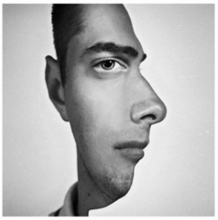
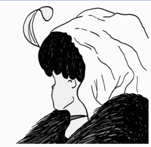
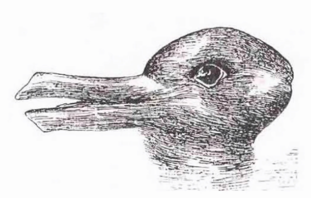
Your brain struggles because it is doing something very specific: it hunts for features. The features closest to your centre of focus win. They decide what you see. The next two illusions make the same point.
And one more. Look at it for just a second. Most people feel almost dazzled. Their eyes jump up and down the face. Both readings seem plausible — so the brain cannot settle on either.
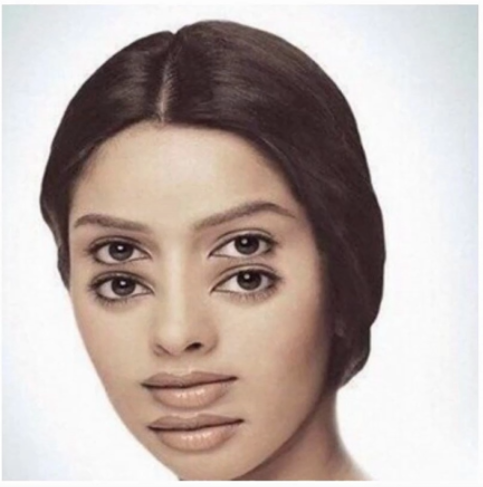
Here is the lesson of the four illusions. Your brain labels what it sees by matching features. The features it picks decide the label. Not enough features, or too little time — and it guesses wrong. You have done this. A quick glance over your shoulder, and a shadow becomes a car. A ball turns out to be a cat.
A convolutional neural network sees in almost the same way. It hunts for small features in an image. It weighs them. Then it outputs a label — with a probability. Keep the illusions in mind through the whole chapter. They are the intuition. The mathematics that follows is the machinery.
2. What a Trained CNN Says
From human brains to machine brains. The slide below comes from a talk by Geoffrey Hinton. It shows three images from a test set — and, under each, a trained network's ranked guesses.
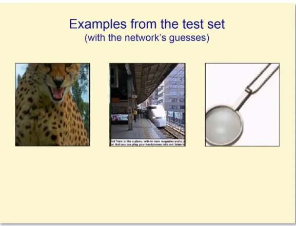
You will meet tables like this everywhere in computer vision, so let us learn to read one properly. The top word is the true label — what the image actually is. Under it come the network's top guesses, ranked, each with a probability. And the network was not choosing among four options. It was choosing among thousands of classes at once.
| True label | The network's ranked guesses | Verdict |
|---|---|---|
| cheetah | cheetah (~95–99%) · leopard · snow leopard · Egyptian cat | right, and confident |
| bullet train | bullet train · passenger car · subway train · electric locomotive | right — telling fine grades of "train" apart |
| magnifying glass | scissors · hand glass (magnifying glass) · frying pan · stethoscope | wrong — but the true answer was a close second |
Read the third row like the illusions of Section 1. The image is genuinely unclear. A human hesitates between a frying pan, scissors and a magnifying glass too. The network hesitated the same way: its probabilities were spread, not peaked. It put scissors first. The true answer came second. That is why the slide marks it in red. A network that hesitates when the image deserves hesitation is a healthy network.
One more thing to hold on to. This slide is years old, and today's networks are far better. By Section 10 you will train your own — and read its ranked guesses on real cat and dog photos.
3. Why CNNs Are Taking Over
Is this field actually going anywhere? Search interest says yes. The screenshot below compares two search terms on Google Trends: convolutional neural network in blue, against artificial neural network in red.
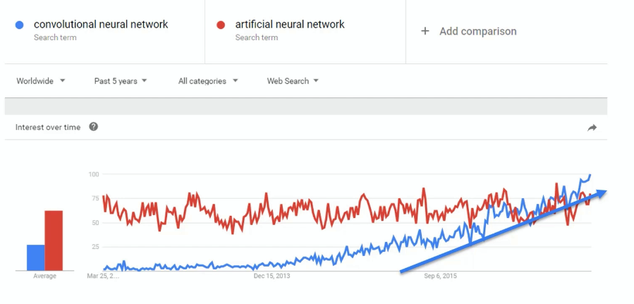
The red line — the general term — stays flat. The blue line climbs from nearly zero and passes it. A specialised term overtaking its own parent field is rare. It says: this is where the energy went.
Where exactly? Self-driving cars: recognising people at the curb and stop signs in a split second. Photo tagging: a few years ago you tagged friends by hand; now faces are found and named for you. Medical scans, factory inspection, satellite images — the same architecture again and again.
4. The People: Hinton and LeCun
Two names stand behind this chapter. If Geoffrey Hinton is the godfather of deep learning, then Yann LeCun is the grandfather of convolutional neural networks. And LeCun was Hinton's student. In the 1980s and 1990s LeCun did the foundational work that made CNNs real. Hinton went on to pioneer deep learning at Google. LeCun became director of AI research at Facebook and a professor at NYU.
5. Pixels as Data
Start at the smallest piece. A black-and-white photo — even one of just 2 × 2 pixels — is a grid of numbers. Each pixel holds one brightness value from 0 to 255. Eight bits, and 28 = 256 options. 0 is a fully black pixel. 255 is a fully white pixel. Everything between is a shade of grey.
A colour pixel holds three such numbers: one for red, one for green, one for blue — RGB. So a colour photo is not one grid but three stacked grids. The computer never sees "colours". It sees ones and zeros bundled into these numbers.
To keep the hand arithmetic readable, this chapter simplifies the range: white becomes 0, black becomes 1. Every rule we compute in this tiny 0/1 world transfers unchanged back to the full 0–255 range. Here is the whole idea in one picture — a smiley face, its pixel grid, and the matrix the network actually receives:
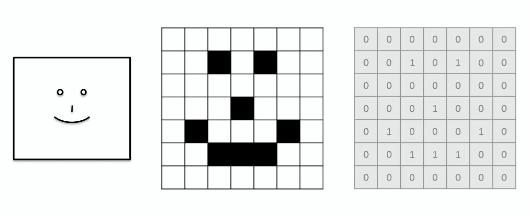
With images as numbers, the whole chapter ahead is four steps: convolution (slide a small pattern across the image to find features), max pooling (keep the strongest finds and shrink the grids), flattening (line the numbers up into one vector), and full connection (a classic Chapter 26 head that makes the final call). Sections 6–7 compute the first two by hand:
To a computer, a photograph is a stack of three grids — red, green, blue — each holding a brightness number per pixel. The network's input here is resized to 64 × 64 × 3 = 12,288 numbers. The task is Chapter 26's shape exactly — binary classification, sigmoid output — but the input is now raw perception, and that changes everything about the architecture.
Why not feed the 12,288 numbers into Chapter 26's Dense network? Two fatal reasons, and they are the chapter's motivation:
- Parameter explosion. A single Dense layer from 12,288 inputs to just 128 neurons owns 12,288 × 128 + 128 = 1,572,992 parameters — before anything has been learned. The entire CNN of this chapter manages the same job with 813,217, of which only 10,144 belong to the two convolution layers that do the actual seeing.
- No translation invariance. A Dense layer learns one weight per pixel-location. A cat in the top-left corner and the same cat one inch to the right hit completely different weights — the network must re-learn "pointy ear" for every position. Vision does not work that way, and neither should our model.
6. The Convolution, by Hand
A convolution slides a small grid of weights — the kernel (or filter) — across the image. At each position it computes one number: the sum of element-wise products between kernel and the patch underneath (exactly the dot product every chapter since Chapter 4 has leaned on). The output grid of all those numbers is the feature map — a map of where the kernel's pattern occurs.
Three names, one thing. The sliding grid is called a kernel, a filter, or a feature detector. All three mean the same small grid of weights. 3 × 3 is the convention. Famous networks break it — AlexNet used 7 × 7, others 5 × 5 — but small kernels dominate. We will use the names interchangeably, and "feature detector" may be the most honest of the three: the grid's whole job is to detect a feature.
6.1 The walkthrough: the smiley, one window at a time
Take the smiley from Section 5 — the 7 × 7 grid of 0s and 1s — and one 3 × 3 feature detector with four 1s in it. The convolution places the detector on the top-left corner of the image. It multiplies each detector value by the pixel underneath it. Then it adds up the nine products. That one sum is the first cell of the feature map:
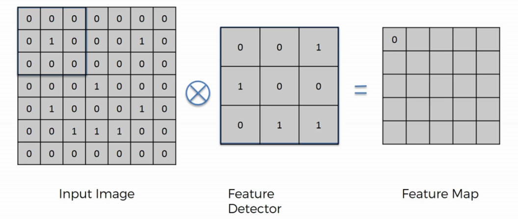
Then it slides. The step size is called the stride. Here the stride is 1: the window moves one pixel to the right, multiplies and sums again, and fills the second cell. At the right edge it drops one row and starts over. A stride of 2 would skip every other position — the map comes out smaller still, and 2 is the common choice in large networks. Slide all the way across and the feature map is complete:
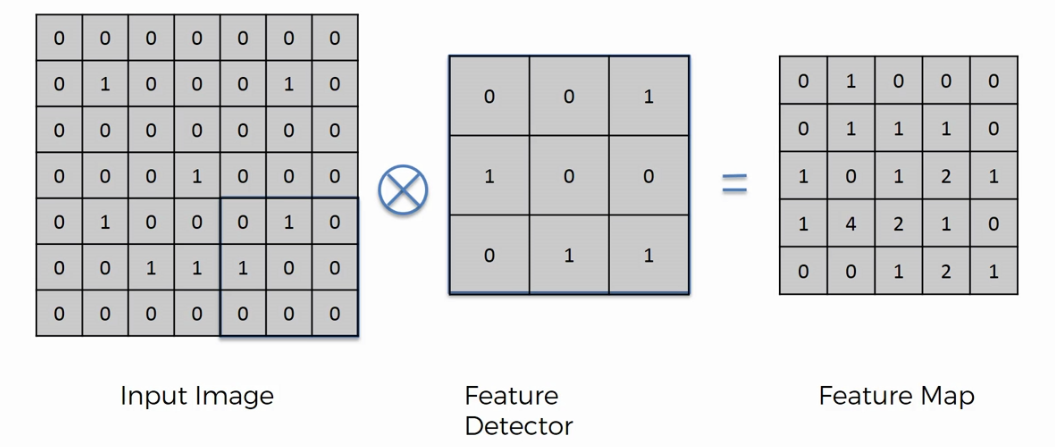
Now read the finished map. Most cells are small — 0, 1, 2. Where the detector's pattern fits nothing, the sum is 0. But one cell holds a 4, the largest value in the map. It sits exactly where the detector matched the image perfectly: all four of its 1s landed on 1s, on the patch straddling the smiley's nose and the left end of its smile (verified by recomputation). That is the whole purpose in one number. The feature map is brightest where the feature lives.
Notice also what the map is not. It is smaller than the image: 7 × 7 became 5 × 5, and a stride of 2 would shrink it further. Do we lose information? Some. But look at what is kept. The map answers "where is this pattern?" — and where is exactly what vision needs. You do not recognise a cheetah by checking every pixel. You recognise the black tear marks under its eyes. Not every pixel of a train — its shape. Your eyes take in gigabytes per second and keep only the features. The convolution is that trick in arithmetic: keep the feature, drop the rest.
6.2 The same operation with real numbers
Watch it work by hand. A 5 × 5 grayscale patch with a vertical edge (bright left, dark right), and a 3 × 3 vertical-edge kernel:
Verify one cell by hand — the top-middle output, from the dashed window (input columns 2–4, rows 1–3):
Three properties make this operation the right tool for vision, and all three are visible in the tiny example:
- Local connectivity: each output number saw only a 3 × 3 patch — vision is local.
- Weight sharing: the same 9 weights produced every cell — "edge-ness" means the same thing everywhere. This is the translation invariance Dense layers lack, and it is why conv1 below has only 896 parameters.
- Learned, not designed: this kernel was chosen by hand for teaching; in the CNN, backpropagation (Chapter 26, unchanged) learns the kernel values from the data. 32 filters per layer means 32 different patterns discovered.
6.3 Many maps make a layer
One detector finds one pattern. A network needs many. So the same image is convolved with many different detectors — each one producing its own feature map. Stack those maps together and you have the convolutional layer:
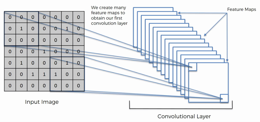
Each map hunts a different pattern — this edge, that curve. Which detectors matter for cats, and which for trains? Nobody assigns them. During training the network decides for itself which features are worth looking for. Section 11 shows the ones our cat-dog network actually learned.
6.4 Kernels you already know
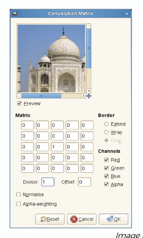
Convolutions are not exotic. Photo editors have used them for decades. These four examples come from the documentation of GIMP, the free image editor: each is a small kernel applied to a photo of the Taj Mahal — exactly our walkthrough, just with real pixel values:
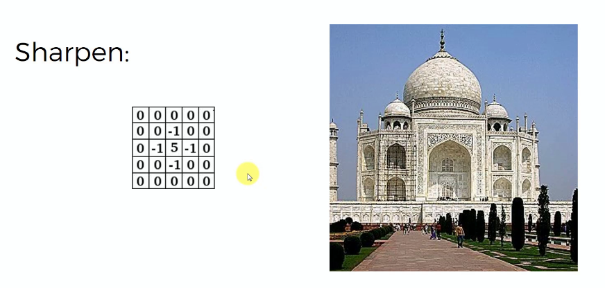
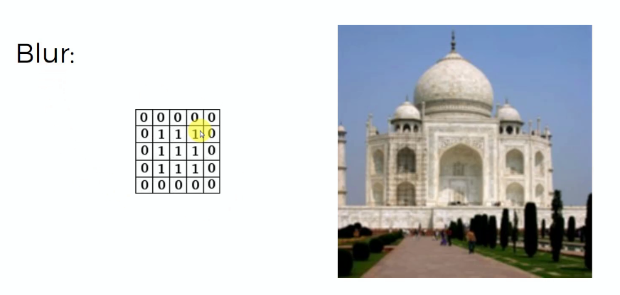
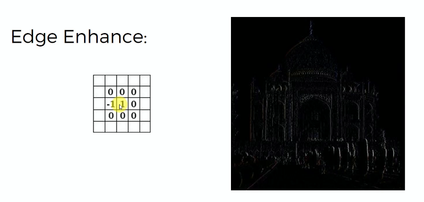
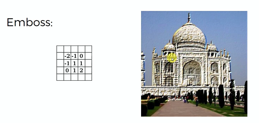
Read each kernel with the walkthrough in mind. Sharpen: the centre pixel is amplified, its neighbours subtracted — edges pop. Blur: equal weights in a block — every pixel is averaged with its neighbours, and differences melt. Edge Enhance: keep the centre, subtract a neighbour — flat areas go dark, boundaries stay bright. Emboss: asymmetric weights, one corner negative and the opposite positive — the photo gains a raised, chiselled look. The cousin that matters most to us is Edge Detect: hunting boundaries is most of what a CNN's early layers do.
And here is the beautiful part. In a trained CNN, nobody designs these kernels. Backpropagation invents them. The learned detectors often look like noise to a human eye and have no name at all — and they work. Section 11 shows our network's own.
6.5 ReLU — breaking the linearity
One small step sits on top of the convolution. It is not a new operation. It is the rectifier — the same activation function Chapter 26 placed inside every neuron. Some courses list it as its own step ("step 1B"). We treat convolution and rectifier as one step, applied to every feature map:
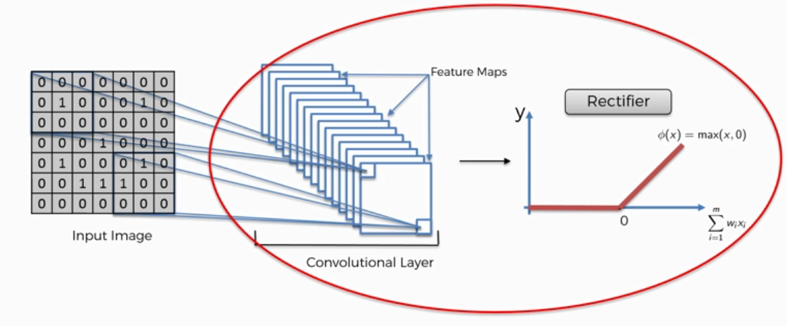
That formula does one thing. Anything negative becomes 0. Everything else stays. Why is this needed? Because the convolution itself is linear: multiply and add, then multiply and add again. Stack linear operations and you get one big linear operation. But images are not linear. Borders, shadows, colour changes — neighbouring pixels jump, they do not slide. A network that can only express straight-line relationships cannot see that. The rectifier breaks the linearity.
Watch it on a real photograph. A city skyline goes through a feature detector. The detector's output is signed: white cells are positive, black cells are negative. Then ReLU removes the black — every negative cell becomes 0:
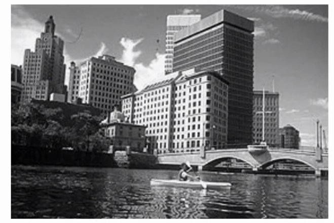
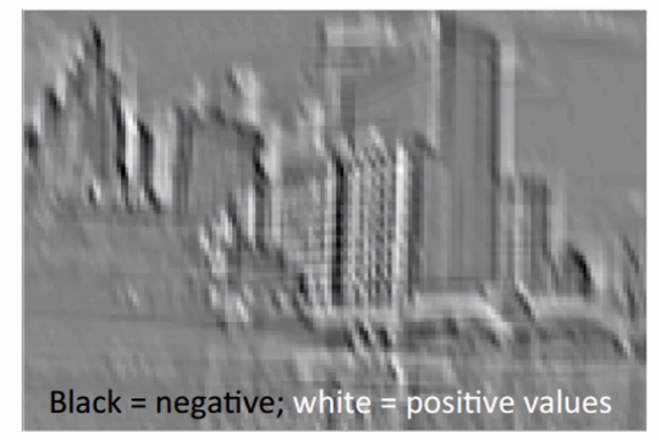
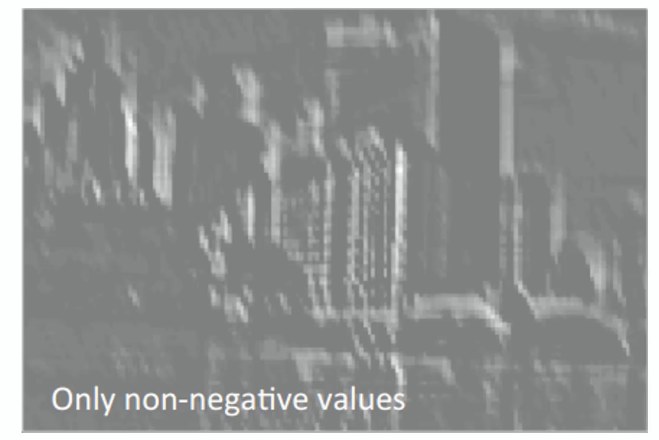
Where exactly is the "breaking" in that? Look at a building's shadow in the middle panel. Bright, then grey, then darker, then black — a smooth, straight-line descent from light to dark. After ReLU the black is cut away. The gradual staircase is gone; what remains jumps abruptly to zero. That abrupt cut is the non-linearity. This is a rough, by-fingers explanation of a mathematical fact — the two papers below make it precise.
And in the code of Section 9 you have already written it,
perhaps without noticing: activation='relu'
rides inside every Conv2D line. Keras has no
separate rectifier layer here — it comes along with the
convolution.
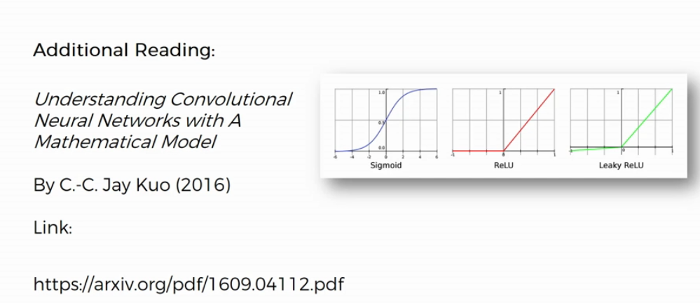
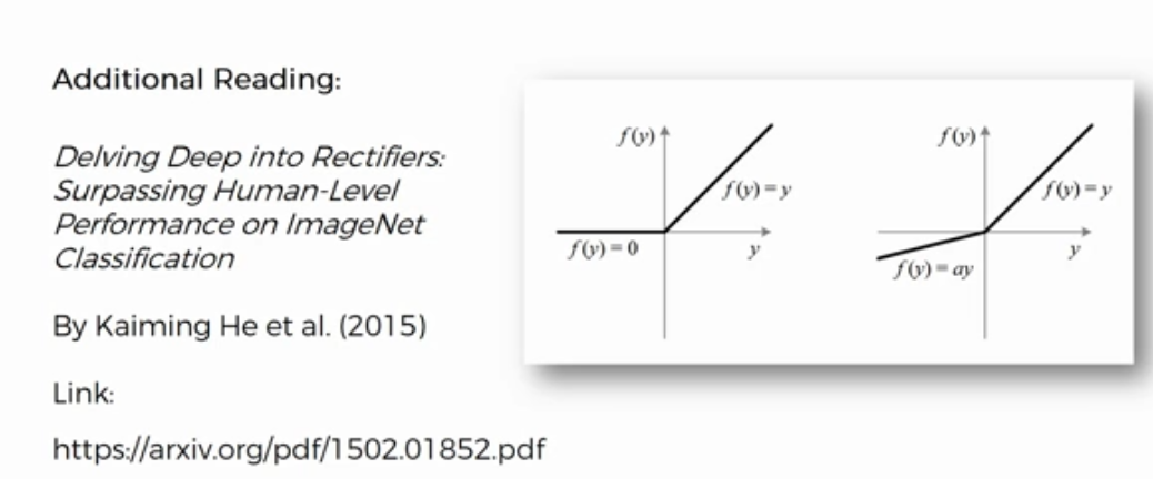
Two papers, if you want to go deeper. The first answers exactly our question — why a non-linear activation is essential at the filter output. The second, from the team at Microsoft Research, proposes a parametric ReLU (PReLU) with a small learnable slope for the negative side — and with it, human-level performance on ImageNet:
7. Pooling & the CNN Architecture
7.1 Max-pooling, by hand
The convolution's companion shrinks the feature map: a 2 × 2 window slides with stride 2, and only the maximum in each window survives. Hand example on a 4 × 4 map:
| Input (4 × 4) | Max-pooled (2 × 2) | |||
|---|---|---|---|---|
| 1 · 3 · 2 · 4 5 · 6 · 7 · 8 0 · 9 · 1 · 2 3 · 4 · 5 · 6 |
→ keep each window's max → |
6 · 8 9 · 6 |
max(1,3,5,6)=6 · max(2,4,7,8)=8 max(0,9,3,4)=9 · max(1,2,5,6)=6 |
|
Two gifts for the price of zero parameters: the map halves in each dimension (fewer numbers downstream), and small shifts of the input barely change the output — the "6" survives whether the 6 sits in its window's corner or centre. Pooling buys tolerance to exact position, which is precisely what a cat that moved two pixels needs.
7.2 The real architecture, layer by layer
Trace the dimensions with the two rules (conv 3 × 3 subtracts 2; max-pool 2 × 2 with stride 2 halves and floors): 64 → 62 → 31 → 29 → 14. Then the 14 × 14 × 32 tensor flattens into a 6,272-long vector, and Chapter 26 takes over: Dense 128 (ReLU), sigmoid output. Every dimension below was verified on the real built model:
| Layer | Output shape | Rule | Parameters |
|---|---|---|---|
| Input | 64 × 64 × 3 | resized photo | — |
| Conv2D, 32 filters, 3×3, ReLU | 62 × 62 × 32 | 64 − 2 = 62 | 3·3·3·32 + 32 = 896 |
| MaxPool 2×2, stride 2 | 31 × 31 × 32 | 62 / 2 | 0 |
| Conv2D, 32 filters, 3×3, ReLU | 29 × 29 × 32 | 31 − 2 = 29 | 3·3·32·32 + 32 = 9,248 |
| MaxPool 2×2, stride 2 | 14 × 14 × 32 | ⌊29 / 2⌋ = 14 | 0 |
| Flatten | 6,272 | 14 × 14 × 32 | 0 |
| Dense 128, ReLU | 128 | full connection | 6,272·128 + 128 = 802,944 |
| Dense 1, sigmoid | 1 | P(dog) | 128 + 1 = 129 |
| Total | count_params() | 813,217 |
Why two conv-pool pairs? Compose the local views: after the first pair, a unit summarises a ~5-pixel patch; after the second, its receptive field has grown again. Early filters detect edges and blobs; later filters combine them into textures and parts — ears, snouts, fur direction. The hierarchy is learned, not designed.
8. Data Augmentation
A photo of a cat is one sample; the same photo slightly
sheared, zoomed, or mirrored is the same cat to any human — and should
be free training data. The ImageDataGenerator creates
these variants on the fly, every epoch:
| Setting | Value | What it does |
|---|---|---|
rescale = 1./255 | ÷ 255 | pixels from 0–255 to 0–1 — Chapter 3's feature scaling, applied to images (both sets) |
shear_range = 0.2 | ±20% | tilts the image, as if photographed at an angle |
zoom_range = 0.2 | ±20% | random zoom in/out — the cat may fill the frame or sit small |
horizontal_flip | True | mirror image — a cat facing left is still a cat |
Augmentation is an overfitting defence: the network almost never sees the same image twice, so it cannot memorise 2,000 photographs — it must learn cat-ness and dog-ness. Section 10's real curves show it working, and also show its limit.
The generators also read the folder structure itself:
flow_from_directory('dataset/training_set') expects one
sub-folder per class (cats/, dogs/) and
infers the labels. The mapping lands in
class_indices — the real run printed
{'cats': 0, 'dogs': 1} (alphabetical) — which makes
the sigmoid output P(dog) exactly.
9. Implementation in Python (Keras)
import tensorflow as tf
from tensorflow.keras.preprocessing.image import ImageDataGenerator

# ---- Part 1: data (augment train, rescale-only test)
train_datagen = ImageDataGenerator(rescale=1./255,
                                   shear_range=0.2,
                                   zoom_range=0.2,
                                   horizontal_flip=True)
training_set = train_datagen.flow_from_directory('dataset/training_set',
                                                 target_size=(64, 64),
                                                 batch_size=32,
                                                 class_mode='binary')
test_datagen = ImageDataGenerator(rescale=1./255)
test_set = test_datagen.flow_from_directory('dataset/test_set',
                                            target_size=(64, 64),
                                            batch_size=32,
                                            class_mode='binary')
print(training_set.class_indices)     # {'cats': 0, 'dogs': 1}

# ---- Part 2: the CNN (813,217 parameters)
cnn = tf.keras.models.Sequential([
    tf.keras.layers.Input(shape=(64, 64, 3)),
    tf.keras.layers.Conv2D(filters=32, kernel_size=3, activation='relu'),
    tf.keras.layers.MaxPool2D(pool_size=2, strides=2),
    tf.keras.layers.Conv2D(filters=32, kernel_size=3, activation='relu'),
    tf.keras.layers.MaxPool2D(pool_size=2, strides=2),
    tf.keras.layers.Flatten(),
    tf.keras.layers.Dense(units=128, activation='relu'),
    tf.keras.layers.Dense(units=1, activation='sigmoid'),
])

# ---- Part 3: compile and train (validate each epoch)
cnn.compile(optimizer='adam', loss='binary_crossentropy', metrics=['accuracy'])
cnn.fit(x=training_set, validation_data=test_set, epochs=25)

# ---- Part 4: a single prediction
import numpy as np
from tensorflow.keras.preprocessing import image
test_image = image.load_img('dataset/single_prediction/cat_or_dog_1.jpg',
                            target_size=(64, 64))
test_image = np.expand_dims(image.img_to_array(test_image), axis=0)
result = cnn.predict(test_image)            # P(dog), since dogs = 1
prediction = 'dog' if result[0][0] >= 0.5 else 'cat'
print(prediction)
Listing 27.1 — The complete cat-dog CNN (source: convolutional_neural_network.py, modernised: Input layer, explicit threshold).
dataset/training_set (8,000 images: 4,000 cats
+ 4,000 dogs), dataset/test_set (2,000) and
dataset/single_prediction/, shipped with the original
course bundle rather than the code repository. This chapter's real
run uses the freely downloadable filtered subset of the same
Kaggle source — 2,000 train / 1,000 test
(cats_and_dogs_filtered.zip, a public mirror such as
the Pytorch-Image-Classification GitHub release) arranged into the
same folder layout. Structure your folders exactly:
dataset/training_set/cats/*.jpg,
dataset/training_set/dogs/*.jpg, and the two
test_set/ equivalents.
# restructure a downloaded filtered subset into the source layout
mkdir -p dataset/training_set dataset/test_set dataset/single_prediction
cp -r cats_and_dogs_filtered/train/cats  dataset/training_set/cats
cp -r cats_and_dogs_filtered/train/dogs  dataset/training_set/dogs
cp -r cats_and_dogs_filtered/validation/cats dataset/test_set/cats
cp -r cats_and_dogs_filtered/validation/dogs dataset/test_set/dogs
Listing 27.2 — Preparing the accessible subset (2,000 train / 1,000 validation images).
10. Training & Results — the Real Run
The honest setup first: the original course bundle's 8,000 training images were not available for this run; the freely downloadable filtered subset (2,000 train, 1,000 test) was trained with the identical architecture, augmentation, and 25 epochs, seed 0. Every number below is that single real run — including the parts that hurt, which turn out to be the best teaching material in the chapter.
| Epoch | 1 | 2 | 3 | 5 | 10 | 15 | 20 | 25 |
|---|---|---|---|---|---|---|---|---|
| Train loss | 0.689 | 0.662 | 0.643 | 0.594 | 0.520 | 0.434 | 0.348 | 0.295 |
| Train acc | 0.554 | 0.629 | 0.633 | 0.681 | 0.735 | 0.802 | 0.843 | 0.884 |
| Val loss | 0.660 | 0.670 | 0.620 | 0.696 | 0.554 | 0.594 | 0.558 | 0.603 |
| Val acc | 0.611 | 0.586 | 0.626 | 0.590 | 0.729 | 0.722 | 0.742 | 0.738 |
Read the two curves the way Chapter 6 taught bias and variance, now in epochs. By epoch 10 the network has learned most of what 2,000 photos can teach: validation loss bottoms at 0.529 (epoch 12). After that, training loss keeps falling — but validation loss climbs (0.554 → 0.603) and validation accuracy merely wobbles around 0.73. That divergence is the real-time signature of the network memorising its training photos instead of generalising: train 0.884 vs validation 0.738 at epoch 25, a 14.6-point gap. The best validation accuracy, 0.742 at epoch 20, marks where training should have stopped — the classic early stopping argument, made by the data.
10.1 The final scoreboard (epoch 25, threshold 0.5)
| Predicted | ||
|---|---|---|
| Actual | Cat (0) | Dog (1) |
| Cat (500) | 341 TN | 159 FP — cats read as dogs |
| Dog (500) | 103 FN — dogs read as cats | 397 TP |
Accuracy 738/1,000 = 0.738; precision 397/556 = 0.714; recall (dogs) 397/500 = 0.794; F1 0.752. The asymmetry is the interesting part: the network finds dogs markedly easier than cats (recall 0.794 vs 0.682 for cats). Cats vary more — posture, flattening, ambiguity — while dog photos in this dataset tend to be more stereotyped (face-forward, tongue out). Real datasets are rarely symmetrically hard; the confusion matrix is where it shows. The probabilities are genuinely confident where correct: min 0.0001, max 1.0000, mean 0.562.
10.2 Single predictions — the source's finale, for real
The source ends by predicting two unseen images one at a time. The real run's answers:
load_img resizes
to 64 × 64, img_to_array makes the 64×64×3 tensor,
expand_dims(..., axis=0) wraps it into a batch of one
(predict always wants a batch), and the raw 0–255 values are
divided by 255 to match training. Skip the rescale and the network
sees an image ten times brighter than anything it trained on.
11. What It Learned, and When CNNs
The two conv-pool pairs are a learned feature hierarchy. Visualising trained filters (or activating images per filter) reliably shows the same progression across CNNs of any size: first-layer filters — direction-selective edges and colour blobs (close cousins of the hand kernel of Section 6, discovered independently by gradient descent); second-layer filters — corners, textures, fur patterns; deeper layers in larger networks — ears, eyes, snouts. The 128-unit Dense layer then plays Chapter 26's role on 6,272 features that actually mean something.
And the honest ledger for this chapter's tool:
| Situation | Right tool | Why |
|---|---|---|
| Images, audio, video | CNN — no serious rival in this course | local structure + translation invariance is what convolutions are |
| Tabular business data | Forests/boosting (Ch 17, 32) | CNNs find no spatial structure in columns; Chapter 26's caveat doubles |
| Text | Embeddings/transformers (Ch 25 §8) | order matters more than locality |
| Huge images, little data | Transfer learning (next section) | never train feature detectors from scratch twice |
12. The Road Ahead
Where image recognition went after this architecture — and why this chapter's from-scratch network is now a teaching artefact rather than a production recipe:
- Deeper, with shortcuts: plain stacks hit limits (vanishing gradients, Chapter 26's enemy); residual networks (ResNet) add skip connections that let dozens or hundreds of layers train — the workhorse backbones of the late 2010s.
- Transfer learning: take a network pretrained on ImageNet's millions of images, freeze its (already excellent) convolutional feature extractors, retrain only the classification head on your 2,000 cats and dogs. Typically beats training from scratch by a wide margin on small datasets — the single highest- value trick in applied vision.
- Attention arrives in vision: vision transformers (ViT) treat an image as patches and apply Chapter 25's attention; hybrid conv+transformer designs dominate current leaderboards. Convolutions remain everywhere — efficient, proven, embedded.
- Data-centric practice: the field's quiet lesson, which this chapter demonstrated live: curated data and augmentation often move the needle more than architecture change.
The course now turns from more data to fewer dimensions. Part IX — Principal Component Analysis first — asks the mirror-image question: when features are many and redundant, which few combinations actually carry the information? Spoiler: eigenvectors, which have been waiting since Chapter 2, finally get their starring role.
🛠 Hands-On: Train, Diagnose, and Improve the DetectorIntermediate
You inherit the cat-dog classifier at 73.8% and one instruction: "make it better, and prove you know why it improved." Walk the full diagnostic path: verify the architecture arithmetic, train, read the curves, stop at the right epoch, then test one improvement.
Steps
- Hand-verify Section 6's convolution (three cells of your choice) and Section 7's max-pool table.
- Hand-verify the dimension chain 64 → 62 → 31 → 29 → 14 and the parameter table; confirm against
count_params()= 813,217 and the per-layer shapes. - Prepare the dataset (Listing 27.2), train for 25 epochs, and reproduce curves shaped like Figure 27.21 (your exact numbers will differ slightly — seed and library builds vary).
- From your curves: locate the minimum validation loss and the best validation accuracy epoch; recommend a stopping epoch with evidence.
- Compute the confusion matrix, accuracy/precision/recall/F1, and the cat-vs-dog recall asymmetry.
- Predict two single images (one cat, one dog) through the full single-prediction plumbing — including the 1/255 rescale — and report the probabilities.
- Improvement test: retrain with
target_size=(128, 128)(adjustinput_shapeaccordingly and re-derive the dimension chain by hand first). Report what moved.
View Solution / Walkthrough
Steps 1–2 (hand): convolution output equals [[0, 30, 30], [0, 30, 30], [0, 30, 30]]; max-pool of [[1,3,2,4], [5,6,7,8], [0,9,1,2], [3,4,5,6]] is [[6, 8], [9, 6]]. Dimensions: 64−2=62; ⌊62/2⌋=31; 31−2=29; ⌊29/2⌋=14. Parameters: 896 + 9,248 + 802,944 + 129 = 813,217.
Step 7 dimension chain at 128 input: 128 → 126 → 63 → 61 → 30 (⌊61/2⌋); flatten 30 × 30 × 32 = 28,800; Dense layer becomes 28,800 × 128 + 128 = 3,686,528 parameters — total ≈ 3.7M, 4.5× the original. Expect a modest accuracy gain at several times the training cost: the compute bill of Section 11, experienced personally.
import numpy as np, tensorflow as tf
from tensorflow.keras.preprocessing.image import ImageDataGenerator
np.random.seed(0); tf.random.set_seed(0)

train_gen = ImageDataGenerator(rescale=1./255, shear_range=0.2,
                               zoom_range=0.2, horizontal_flip=True)
train = train_gen.flow_from_directory('dataset/training_set',
        target_size=(64,64), batch_size=32, class_mode='binary')
test = ImageDataGenerator(rescale=1./255).flow_from_directory(
        'dataset/test_set', target_size=(64,64), batch_size=32,
        class_mode='binary', shuffle=False)

cnn = tf.keras.models.Sequential([
    tf.keras.layers.Input(shape=(64,64,3)),
    tf.keras.layers.Conv2D(32, 3, activation='relu'),
    tf.keras.layers.MaxPool2D(2, 2),
    tf.keras.layers.Conv2D(32, 3, activation='relu'),
    tf.keras.layers.MaxPool2D(2, 2),
    tf.keras.layers.Flatten(),
    tf.keras.layers.Dense(128, activation='relu'),
    tf.keras.layers.Dense(1, activation='sigmoid')])
print('params', cnn.count_params())          # 813217

cnn.compile(optimizer='adam', loss='binary_crossentropy', metrics=['accuracy'])
h = cnn.fit(train, validation_data=test, epochs=25, verbose=0)
va = h.history['val_accuracy']
print('best val_acc %.3f at epoch %d' % (max(va), int(np.argmax(va))+1))

probs = cnn.predict(test, verbose=0).ravel()
y = test.classes; yp = (probs >= .5).astype(int)
from sklearn.metrics import confusion_matrix, accuracy_score
print(confusion_matrix(y, yp), accuracy_score(y, yp))

from tensorflow.keras.preprocessing import image
img = image.load_img('dataset/single_prediction/cat_or_dog_1.jpg',
                     target_size=(64,64))
arr = np.expand_dims(image.img_to_array(img)/255.0, axis=0)
print('P(dog) %.4f' % cnn.predict(arr, verbose=0)[0][0])
Expected results (real canonical run, seed 0): class_indices {'cats': 0, 'dogs': 1}; 813,217 params; best val_acc 0.742 at epoch 20; min val_loss 0.529 at epoch 12; epoch-25 train 0.884 vs val 0.738 (the overfitting gap); CM [[341, 159], [103, 397]], acc 0.738, P 0.714, R 0.794, F1 0.752; cat recall 0.682 vs dog recall 0.794; singles: dog → P(dog) 1.0000, cat → 0.0588. Your run will land near these values but not on them — CPU TensorFlow is nondeterministic across builds; the shape of the story (fast early gains, val plateau, growing gap) is the reproducible part.
🎯 Key Takeaways
Dense layers break on images: 1.57M parameters to connect 12,288 pixels to 128 units, and a weight per location — no translation invariance.
A convolution slides one small learned kernel everywhere: hand example 5×5 ⊛ 3×3 → 3×3 map that lights up (30) exactly on the edge. Same 9 weights, every position.
Max-pooling halves the map with zero parameters and buys position tolerance: [[1,3],[5,6]] → 6. Dimension chain: 64 → 62 → 31 → 29 → 14.
813,217 parameters — but 98.8% sit at Flatten→Dense; the two convolutions that do the seeing own only 10,144. Stack convs to shrink that junction.
Augment training images (shear, zoom, flip — never the test set): the network can't memorise 2,000 photos it never sees twice.
The real run overfit honestly: train 0.884 vs val 0.738; best val 0.742 at epoch 20 → early stopping. Dogs easier than cats (0.794 vs 0.682 recall). Data beats architecture at small scale.
Test Your Understanding
35 questions across the chapter — features and illusions, ranked guesses, pixels, the smiley walkthrough, the hand convolution, kernels, ReLU, pooling, architecture arithmetic, augmentation, and the real training run. Choose one answer per question, then check your answers.
Q1.The dataset and task:
Q2.A 64 × 64 RGB image arrives as:
Q3.Why not feed pixels into Chapter 26's Dense network?
Q4.A convolution is best described as:
Q5.(Hand) In Section 6's example, the top-middle feature-map cell equals 30 because:
Q6.The 9 kernel weights in a real CNN come from:
Q7.(Hand) A 3 × 3 kernel (no padding, stride 1) on a 5 × 5 input produces:
Q8.Weight sharing means:
Q9.(Hand) Max-pool 2×2, stride 2 on [[1,3,2,4],[5,6,7,8],[0,9,1,2],[3,4,5,6]] gives:
Q10.What max-pooling buys:
Q11.(Hand) After conv(3×3) → pool(2×2) → conv(3×3) → pool(2×2) on a 64 × 64 input, the map is:
Q12.Of the CNN's 813,217 parameters, where do they live?
Q13.conv1's 896 parameters decompose as:
Q14.The Flatten layer's job:
Q15.Data augmentation (shear 0.2, zoom 0.2, horizontal flip) exists to:
Q16.rescale = 1./255 is:
Q17.The test generator rescales but never shears/zooms/flips because:
Q18.With class_indices {'cats': 0, 'dogs': 1}, the sigmoid output means:
Q19.The single-prediction pipeline load_img → img_to_array → expand_dims → /255:
Q20.Why expand_dims(arr, axis=0) before predicting?
Q21.(Real) The training curves of Figure 27.21 show:
Q22.(Real) Validation loss was lowest at epoch 12 (0.529) and best validation accuracy was 0.742 at epoch 20. The right conclusion:
Q23.(Real) The confusion matrix [[341, 159], [103, 397]] says:
Q24.(Real) The two single-image predictions came out:
Q25.The noisy validation curve (0.729 → 0.641 → 0.739 across epochs 10–12) is explained by:
Q26.Stacking two conv-pool pairs (rather than one) gives:
Q27.Raising target_size to 128 × 128 would:
Q28.For tabular business data (say, churn), the right tool is:
Q29.Transfer learning, the highest-value trick on small image datasets:
Q30.Chapter 28 (PCA) will ask the mirror-image question of Part VIII's:
Q31.The optical illusions that open the chapter (the hybrid face, the duck-rabbit) teach one specific lesson:
Q32.In a colour image, one pixel is stored as:
Q33.The stride of a convolution is:
Q34.(Hand) In the smiley walkthrough, the feature map's largest value (the 4) appears where:
Q35.The rectifier (ReLU) applied on top of the convolution: